popgen-evomics

1. Allele frequencies and Allele Frequency Spectrum (AFS)

Allele frequency is a frequency of given variant in a population. The Allele Frequency spectrum (AFS, or Site Frequency Spectrum) is a histogram that describes the number of genetic variants with a given frequency in a set of sequences. It can be used to estimate the dynamics of the population (expansion, bottleneck etc.).

In this part of the tutorial, we are going to learn how to analyze and show the differences in allele frequencies between Africans and Americans individuals in the HPRC dataset. By the end of this tutorial, we should have a graph that shows how these gene frequencies vary between the two groups, e.g. which population is enriched for rare variation, giving us a concise picture of genetic diversity betwee these two populations.

We will learn how to:

(a) calculate allele frequencies using plink2
(b) calculate population-specific allele frequencies
(c) how to bin allele frequencies to plot the allele frequency spectra (AFS)

Navigate to the folder `1_afs` within the `mytutorial` folder

cd mytutorial
cd 1_afs

(a) Overall allele frequencies and histogram of allele counts

Calculate allele frequencies directly from vcf, only for the SNPs, for all samples.

plink2 --vcf /home/genomics/workshop_materials/population_genomics/chr15.pan.fa.a2fb268.4030258.6a1ecc2.smooth.reliable.vcf.gz \
       --freq \
       --allow-extra-chr \
       --vcf-half-call m \
       --snps-only \
       --out chr15

## --vcf loads a genotype VCF file
## --allow-extra-chr  force to accept chromosome code 'chm13#chr15'
## --vcf-half-call specify how GT half-call should be processed. See tutorial section 0 for more info
## --snps-only  selects only loci that are single nucleotide polymorphisms 
## --out gives a human-readable name 

This command will produce these files:

-rw-rw-r-- 1 enza enza 33492352 gen 14 11:28 chr15.afreq
-rw-rw-r-- 1 enza enza      923 gen 14 11:28 chr15.log

Open the .log file and read it to check that all went well.

Open the .afreq file and look at it. Check the info on the content of the columns and get familiar with it:

cat chr15.afreq | column -t | less -S 

Can you guess why for some loci the allele frequency is null (nan)?

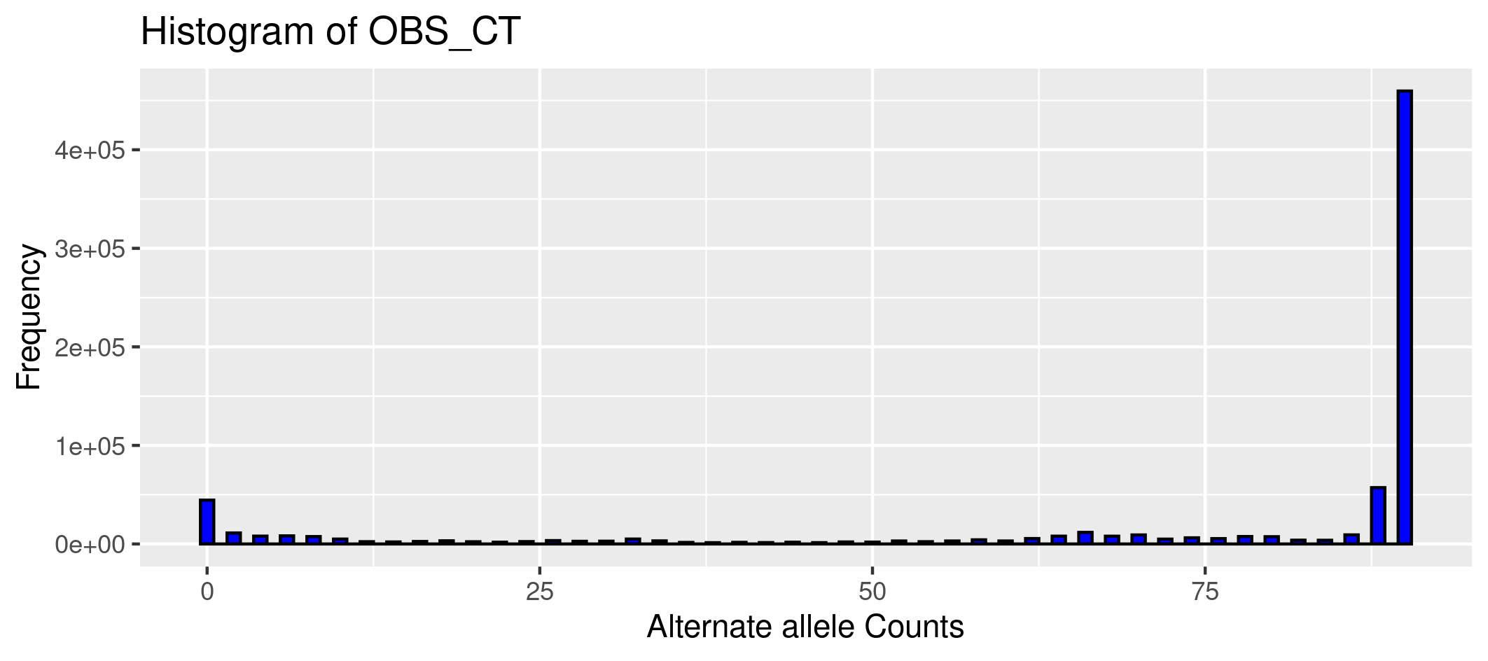
Plot the counts of the alternate allele to obtain the allele frequency spectrum from the alternate allele counts:

 Rscript  ../../rscripts/1.plotafsCOUNTS.R chr15.afreq HPRC-allele-counts

## first argument is the file with the allele counts 

## second argument is the title of the graph

Open the file with the plot:

afscount

(b) Population-specific allele frequencies

Next we want to calculate allele frequencies specifically for the African and American populations. This time we will use the plink2 fileset instead of the vcf.

The crucial first step involves identifying the samples that belong to these specific populations. This information is in metadata files that we need to reference using the --keep option:

plink2 --pfile  ../data/chr15 \
       --keep  ../../metadata/afr.onlyid \
       --freq \
       --allow-extra-chr \
       --snps-only \
       --out chr15.afr 

plink2 --pfile  ../data/chr15 \
       --keep  ../../metadata/amr.onlyid \
       --freq \
       --allow-extra-chr \
       --snps-only \
       --out chr15.amr 

## --pfile specifies which plink2 file set to use, you only need to specify the file prefix (e.g. chr15) 
## --keep reference to the file containing the individuals to filter for (i.e. keep only individuals listed in the file)
## Note that we are filtering for individuals from African (afr) and the Americas (amr).

This will produce:

-rw-rw-r-- 1 enza enza 32483032 gen 14 11:38 chr15.afr.afreq
-rw-rw-r-- 1 enza enza      863 gen 14 11:38 chr15.afr.log
-rw-rw-r-- 1 enza enza 30547659 gen 14 11:38 chr15.amr.afreq
-rw-rw-r-- 1 enza enza      863 gen 14 11:38 chr15.amr.log

As usual, open the log and check for error messages if any. Open the .afreq files and look at the content

(c) Allele Frequency Spectrum (AFS) of multiple populations

To produce the AFS we should bin the allele frequencies in classes. In plink2, the --freq option includes the refbin (bin by the reference allele) and alt1bin (bin by the alternative allele) modifiers for generating histogram counts during allele frequency calculations. To use these modifiers, you must specify the bin intervals either directly in the command line or by referencing a file, and using the refbin-file and alt1bin-file modifiers.

We can produce the bin info file with a simple shell command that write a sequence form 0.1 to 1 in intervals of 0.05 and store it in a file called mybins.txt:

LC_NUMERIC="C" seq -s " " 0.05 0.05 1.0 > mybins.txt

Look at the mybins.txt file so you better understand what the code above did:

cat mybins.txt

Calculate the counts for the AFS based on alternate allele frequencies:

plink2 --pfile  ../data/chr15 \
       --keep  ../../metadata/afr.onlyid \
       --freq alt1bins-file='mybins.txt' \
       --allow-extra-chr --snps-only \
       --out chr15.afr

plink2 --pfile  ../data/chr15 \
       --keep  ../../metadata/amr.onlyid \
       --freq alt1bins-file='mybins.txt' \
       --allow-extra-chr \
       --snps-only \
       --out chr15.amr

## --freq alt1bins-file='mybins.txt' specify to bin the frequency as described in the file mybins.txt 

These commands will produce:

-rw-rw-r-- 1 enza enza      213 gen 16 09:43 chr15.afr.afreq.alt1.bins
-rw-rw-r-- 1 enza enza      212 gen 16 09:43 chr15.amr.afreq.alt1.bins

Look at the files chr15.afr.afreq.alt1.bins and chr15.afr.afreq.alt1.bins. To plot the AFS, we will use R. You can load the two files in Rstudio and write your own code (using ggplot - from what you learned earlier in the week!) or use the pre-prepared R script 1.plotafs.R in the ../../rscripts folder. Note that you can use the Rscript command to execute R scripts directly from the command line without the need for an interactive R environment.

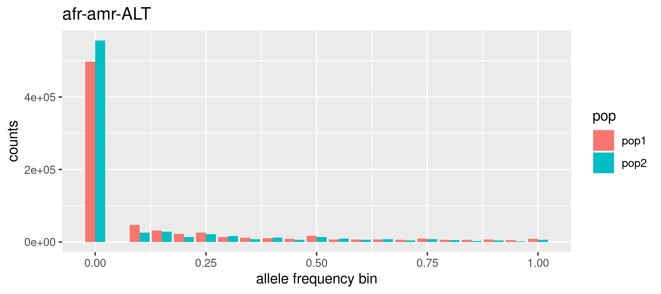
Rscript ../../rscripts/1.plotafsFREQ.R chr15.afr.afreq.alt1.bins chr15.amr.afreq.alt1.bins afr-amr-ALT

# first argument is the allele frequency in the first population 

# second argument is the allele frequency in the second population 

# third argument is the title of the graph, I chose afr-amr to remember the name of the populations and ALT
# to remember that we are considering the Alternate allele frequency. Do not use spaces if multiple words! 

Look at the png file just produced. To view the png image, you can use Guacamole desktop or copy the file to your laptop using scp command. afs

Which population is enriched for rare variants? Can you guess why?

Back to sections